A European options contract gives the buyer the right, but not the obligation to buy or sell an asset at a predetermined strike price at expiry. The payoffs are asymmetric: the maximum loss is capped at the market value of the option (known as the premium), whereas the potential gains are in theory unlimited, depending on how far the prices drift away from the strike.
Understanding the factors that matter when pricing options is a crucial step to grasping their market dynamics. Implied volatility (IV) is the central variable to be considered, expressing the market-implied expectation of future price diffusion in the underlying asset.
In option markets, IV has become one of the most closely monitored metrics to the extent that it has replaced the spotlight traditionally taken by price. To see why this is the case, imagine 2 stocks trading at $100, with call options struck at $110. The first option A and second option B have an IV of 2%, and 10% respectively. B has a higher IV than A, reflecting a larger expected dispersion of future underlying prices. As a result, the probability of extreme outcomes increases, making B more valuable and expensive than A. This example is reflective of a broader intuition that the price of an option tends to be highly, though partially, driven by IV. Traders are willing to pay more when the distribution of possible outcomes is wider, as this increases the possibility of more significant moves that can generate disproportionately large profits.
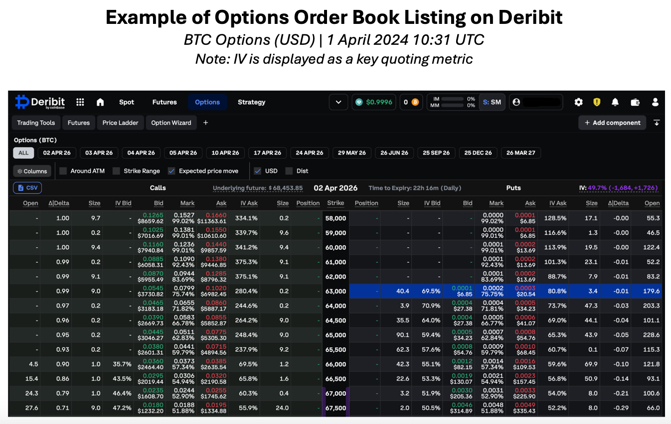
IV is the preferred quotation mark for pricing crypto contracts because it has an intuitive, standardised interpretation that can theoretically strip the noise away. The premium of $100 tells you very little about the desirability of A and B without further information, whereas the 2% and 10% IVs reflect relative value under a unique figure that is comparable across strikes, expiries and different asset classes. This can be seen in the fact that IV is often the primary variable in trading communication and order book listings on option trading platforms. Options are quoted and traded in IV terms, rather than in premium or dollar terms (“options trades at 60% IV”). When a trader says an option is “cheap” or “expensive”, they typically mean relative to IV, not to its dollar price.
As a rule of thumb, implied volatility, option demand, premium (option price) and the market sentiment tend to be positively correlated. Higher IV typically corresponds to contracts that are more desirable as there is potential for larger profits. In consequence, the premium increases in puts and conveys a bearish market sentiment.
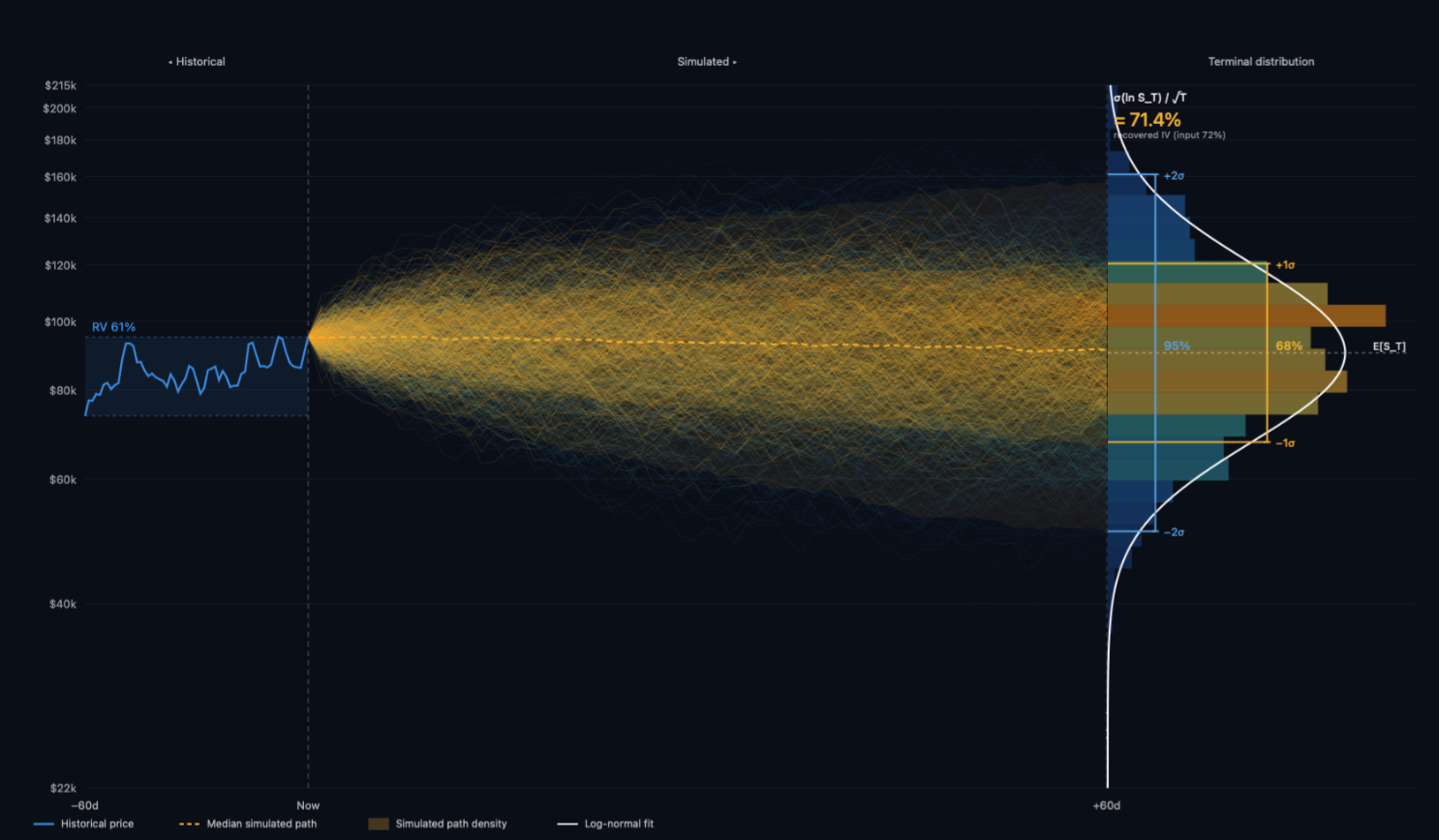
The word “implied” rather than “expected” is used deliberately, indicating the method by which these volatilities are obtained. Unlike traditional volatilities estimated from historical data, implied volatilities can be inferred from the current market prices of financial instruments.
Using the market price as the derivation point for the IVs is internally consistent with market conditions reflecting participants’ positions, hedging needs, event risk, sentiment, right now. IV effectively becomes a pseudo-sentiment indicator, as traders are watching for IV levels to gauge market fear or complacency. Historical data may inform those prices, but IV reflects better the market’s statement today in expectation of tomorrow.
Option pricing and the derivation of IV are often stated in conjunction with the Black-Scholes-Merton (BS) model. The BS model was originally designed to price any derivative that is dependent on a non-divident paying stock, which sits well in a crypto option market context.
The idea behind BS is setting up a riskless portfolio consisting of a position in the derivative and an offsetting position in the underlying asset. Since the derivative and the underlying are driven by the same source of uncertainty, namely the asset’s price movements, their values are perfectly correlated over a split-second period of time. The correlation is captured by delta, the sensitivity of the option’s price to a unit change in the underlying, the hedge ratio when constructing the portfolio.
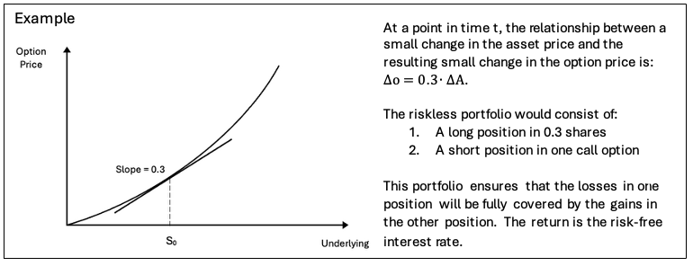
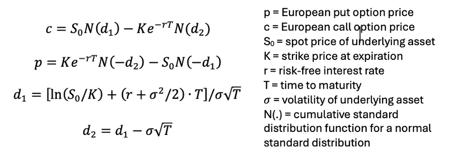
To remain riskless throughout time, this portfolio requires dynamic rebalancing. By adjusting the derivative price and the delta units of the underlying to the appropriate proportions, the exposure to price movements cancels out, resulting in a position that is momentarily riskless. In the absence of arbitrage opportunities, such a portfolio must earn exactly the risk free rate of return. BS’s no-arbitrage condition pins down the fair value of the derivative, from which the pricing closed-form solutions for the call and put European options are derived:
To explain one of the two intuitively, the call’s price formula can be seen as an adaptation of the classic “if-else” payoff structure:
This function indicates that the option only has value if the stock price exceeds the strike at maturity. In practice, options hold value before maturity based on the expected future payoff under uncertainty. The Black-Scholes model captures this by introducing a continuous “present-value” type of function, which requires the use of probabilities and time-induced discounting.
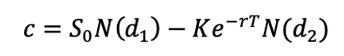
This expression can be interpreted as the expected benefit of receiving the underlying minus the expected cost of exercising the option, adjusted for probability and time value.
The variables d1 and d2 both measure the gap between the underlying price and the strike price (ln(S0/K)), adjusted for time, interest rate and volatility. Both variables are standardized so that they follow a standard normal distribution, which allows the cumulative distribution functions N(.) to convert them into risk-neutral probabilities to be then used in the pricing formula.
The term d2 is associated with the strike price component of the call formula, where N(d2) represents the risk-neutral probability that the option will be exercised (ST > K). In contrast, d1 is linked to the underlying price component, where N(d1) reflects the option’s sensitivity (delta) to changes in the underlying asset price. IV affects how the risk-neutral probabilities are formed, shaping the dispersion of future prices.
Since the strike price term represents a potential future payment, it must be reverted to its present value, which justifies the presence of the time-discounting factor e-rt. The exponential term is used rather than discrete discounting such as (1+r)-t because the Black Scholes model assumes compounding of the risk free rate within a continuous time framework, which ensures consistency with the other assumptions of the model.
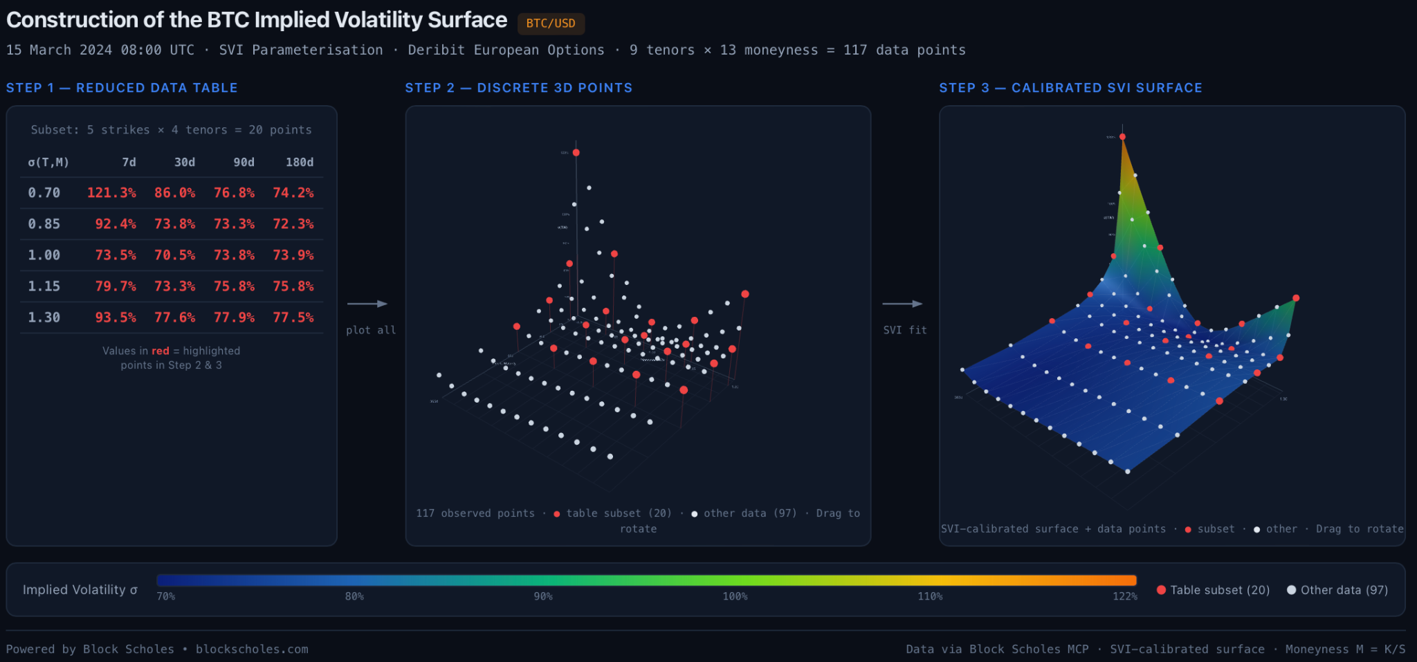
A simple way of thinking about the IV surface is as a continuous representation of implied volatilities across three dimensions: strike or moneyness, time to expiry and volatility points. The surface provides a consistent view of how the market prices uncertainty across different option contracts at any given point in time.
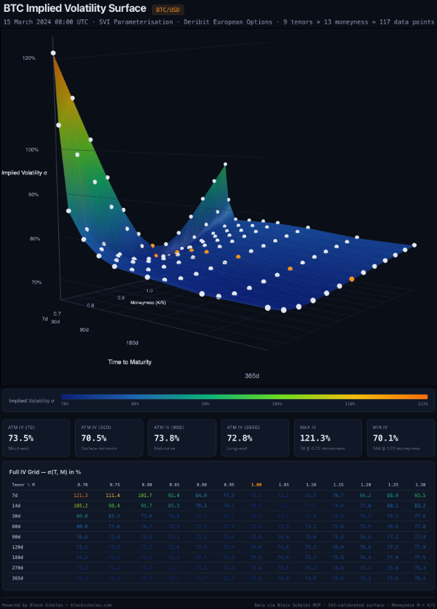
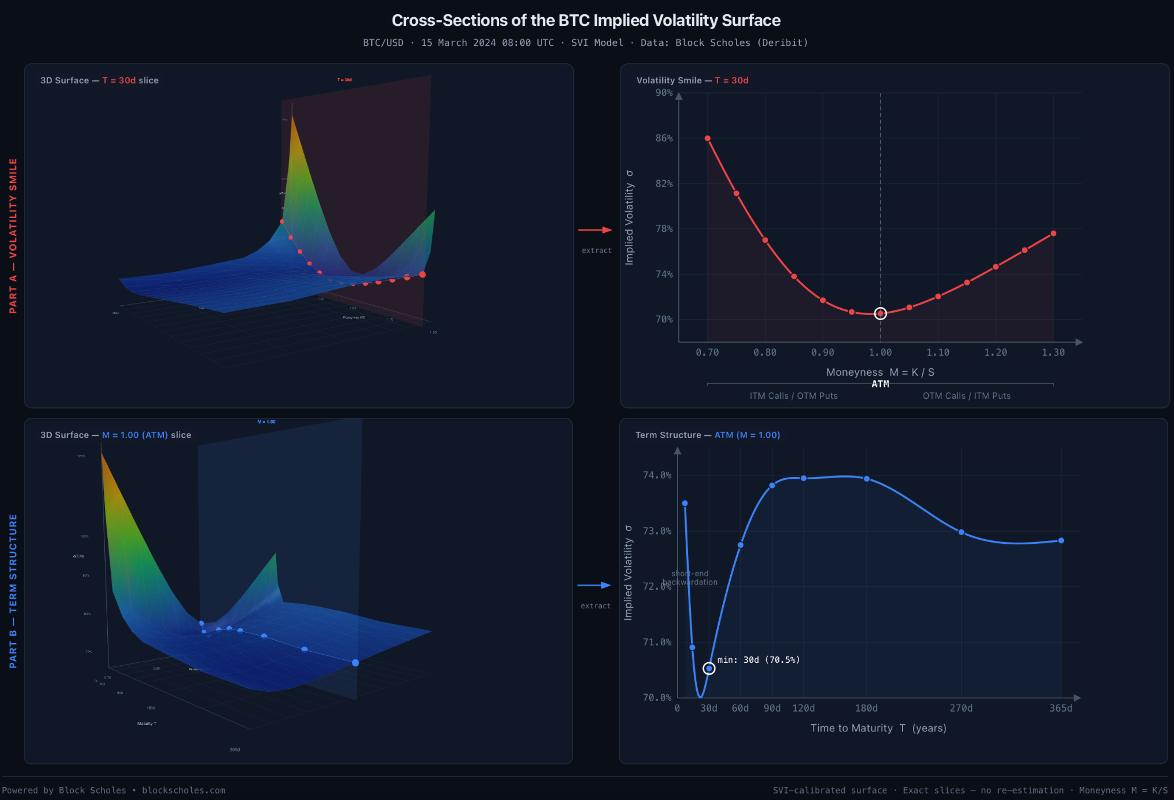
In practice, the surface is not observable in continuous form and must be constructed from discrete option prices. This is typically achieved by calibrating parametric models such as the Stochastic Volatility Inspired (SVI) model to market data, resulting in a smooth surface. When properly specified, the IV should depend on only a small number of parameters and be consistent with the no-arbitrage condition, preparing the groundwork for accurate and flexible option pricing.
Once calibrated, the surface becomes a compressed representation of the entire options market, allowing traders to re-price any real or theoretical option at any point in time using a standard model like Black Scholes, recovering a price consistent with what the market was implying at the time. In crypto derivatives markets, this makes the volatility surface a central reference system for pricing, hedging and relative value analysis.
Backtesting is a crucial step in developing an options trading strategy, evaluating how it would perform on historical data before live trading under real market conditions. Unlike equity trading strategies where a backtest can be run directly on historical price series, options backtesting requires an additional layer of complexity because each option is a different instrument whose value depends non-linearly on multiple inputs. Options may also not trade every day or have missing or stale prices. Since raw prices tend to be sparse, noisy and inconsistent across strikes and maturity, they ought to be derived instead from a calibrated IV surface.
Examples of crypto trading strategies using IV include:
Despite the various implementations, IV-based backtests share a common structure: IV serves as the input signal observed at each point in time, the trading rules map the signal into position decisions, and the simulation plays out using historical option prices and underlying asset data. The aim is to determine whether IV contains any predictive information about future realised volatility or option mispricing.
We explore one implementation of these strategies “by hand” and by using Block Scholes’ own backtester in our next article, Trading Strategy Backtest Implementation.
In any financial contract where two parties agree to conditional future payments, there should be a way of protecting against the possibility that the risk-bearing party cannot fulfill their obligation. This applies to crypto derivatives, where each option contract that is written or sold requires a margin that the seller must have in place.
Stock margins are calculated as a percentage of their market value. As option pricing depends on multiple factors, percentage-based margining used for linear instruments is not an appropriate method. Instead, option margins are designed such that they can absorb potential worst-case losses on a position resulting from evolving market conditions, based on a risk-based framework.
IV is central in this process, used to generate price shock scenarios for the underlying asset. Exchanges typically maintain a full volatility surface and perform stress tests by simulating changes in both the underlying and the volatility. For each test, the option’s position is reevaluated and the resulting loss is computed. The margin is set equal to the maximum loss across these scenarios.